The Deep of Deep Learning

Deep learning is a machine learning sub-branch that can automatically learn and understand complex tasks using artificial neural networks. Deep learning uses deep (multilayer) neural networks to process large amounts of data and learn highly abstract patterns. This technology has achieved great success in many application areas, especially in image recognition, natural language processing, autonomous vehicles, voice recognition, and many more.
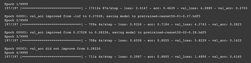
The term “epoch” is used when training deep learning models. An epoch is an iteration period in which the model processes the training data. During each epoch, the model reviews the data, makes predictions, and calculates how well these predictions match the actual values. It then calculates the measure of this mismatch using a loss function.
The epoch number is a factor that affects the model’s ability to learn from the data. The model may make more errors in the first epochs but learns to make better predictions over time. However, using too many epochs can lead to overfitting, i.e., the model fits the training data very well, but the ability to generalize to new data is reduced.
Deep learning can require large datasets and high computational power, so it is often used in large-scale applications. However, this technology offers important innovations and solutions for many fields and is a rapidly developing research and application area.
Epoch
An epoch is a complete pass a deep learning model spends over the dataset once during training. A dataset consists of data that contains information from which the model can learn and improve its predictions.
What Occurs During an Epoch?
During an epoch, the model makes predictions for each sample in the dataset, and loss values are calculated using a loss function that measures the accuracy of these predictions. The model weights are updated according to these loss values and thus aim to make the model predictions more accurate.
During training, the model goes through multiple epochs. During each epoch, the model aims to learn to make better predictions on the dataset. Closer to the completion of the training process, the model’s predictions usually become closer to the expected outputs, and the loss values decrease.
During training, the number of epochs can affect the model’s performance. If too many epochs are used, the model will overfit and may perform well on the dataset but underfit (overfit) when applied to new data. If too few epochs are used, the model may not learn enough or reach the expected outputs (underfitting). Therefore, keeping the epoch count at an accurate level is essential to optimize the model’s performance.
Loss Function
In deep learning models, the loss function measures the degree to which models can make accurate predictions. For example, when a neural network model tries to predict the label of an image, the loss function measures the accuracy of the model’s predictions. It helps to correct the model’s predictions.

Loss functions are usually scalar values that measure how much the models’ output differs from the expected output. This difference shows how accurate the models’ predictions are. Low loss values indicate that the model makes better predictions, while high loss values suggest that the model makes worse predictions.
The loss functions are calculated automatically during the model’s training and aim to correct the model’s weights. Updating the weights of the model makes the model’s predictions more accurate. This process is performed using an optimization algorithm called backpropagation. This algorithm calculates how the model should correct the weights to reduce the loss function and updates the model weights accordingly.
The following criteria can also be considered when choosing the loss function:
- The application for which the model is intended: The appropriate loss function can be selected according to which application the model will be used. For example, a loss function such as cross-entropy loss can be utilized in a classification problem. However, in a regression problem, a loss function such as mean square error can be used.
- Properties of the dataset: The appropriate loss function should be selected for whatever data type is contained. For example, a loss function such as cross-entropy loss can be used in classification problems. In regression problems, a loss function such as mean square error can be utilized.
- The accuracy of the model’s predictions: The choice of the loss function is also essential to measure the accuracy of the model’s predictions. For example, a loss function such as cross-entropy loss is used to calculate the accuracy of forecasts in classification problems. However, a loss function such as the mean square error is used to measure the accuracy of the estimates in regression problems.
- Size of the dataset: The size of the dataset is also essential in the selection of the loss function. For example, a loss function such as mean square error can be used in large data sets. However, a loss function such as cross-entropy loss may be more appropriate for small datasets.
- Model performance: The loss function selection is also essential to measure the model’s performance. For example, in a classification problem, measuring the model’s performance using a loss function such as cross-entropy loss may be more accurate. However, in a regression problem, measuring the model’s performance using a loss function such as mean square error may be more precise.
Some commonly used loss functions are:
Mean Squared Error (MSE):
- Used for regression problems.
- Measures the average squared difference between predicted and actual values.
- Formula: MSE = (1/n) * Σ(actual — predicted)²
Binary Cross-Entropy Loss (Log Loss):
- Used for binary classification problems.
- Measures the dissimilarity between the true binary labels and predicted probabilities.
- Formula: BCE = -Σ(y * log(p) + (1 — y) * log(1 — p)), where y is the true label, and p is the predicted probability.
Categorical Cross-Entropy Loss (Softmax Loss):
- Used for multi-class classification problems.
- Measures the dissimilarity between the actual class labels and predicted class probabilities.
- Formula: CCE = -Σ(y_i * log(p_i)), where y_i is the true label for class i, and p_i is the predicted probability for class i.
Hinge Loss (SVM Loss):
- Used for support vector machine (SVM) and binary classification problems.
- Maximizes the margin between classes by penalizing misclassified samples.
- Formula: Hinge Loss = max(0, 1 — (y * f(x))), where y is the true label (-1 or 1), and f(x) is the decision function.
Huber Loss:
- Used for regression problems, particularly robust to outliers.
- Combines the advantages of MSE and Mean Absolute Error (MAE).
- Formula: Huber Loss = Σ(|actual — predicted| <= δ) * 0.5 * (actual — predicted)² + Σ(|actual — predicted| > δ) * δ * |actual — predicted|
Kullback-Leibler Divergence (KL Divergence):
- Used in probabilistic models and for measuring the difference between two probability distributions.
- Measures how one distribution diverges from another.
- Formula: KL(P || Q) = Σ(P(x) * log(P(x) / Q(x))), where P and Q are probability distributions.
Triplet Loss:
- Used in triplet networks for face recognition and similarity learning.
- Encourages the embedding of anchor samples closer to positive samples and farther from negative samples.
- The formula varies depending on the specific variant.
These are just a few examples, and many other loss functions are designed for specific tasks and scenarios in machine learning and deep learning. The choice of a loss function depends on the nature of the problem you are trying to solve.
Optimizer:
Optimizer is a component used to update parameters (such as weights and biases) in machine learning and deep learning models and optimize the training process. The optimizer adjusts the parameters to minimize the error calculated by the loss function.
The optimizer updates the internal parameters of the model based on the error calculated by the loss function. These updates are made to minimize loss and improve the model’s performance. The optimizer calculates gradients (slopes) using backpropagation and updates parameters using these gradients.
- The Loss function calculates an error value by comparing the model’s predictions with the actual labels.
- The optimizer calculates this error value and the gradients of the parameters inside the model.
- Gradients ensure that parameters are updated in the right direction.
- The optimizer applies these updates to the model’s parameters.
- This process is repeated to minimize the value of the loss function and make the model perform better.

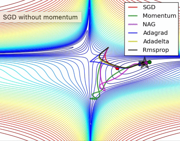
The optimizer and loss function work together to optimize the model’s training. Different optimization algorithms (e.g., Gradient Descent, Adam, RMSprop) can perform parameter updates differently, affecting the model’s training. Choosing a good optimizer can help the model achieve faster and better results.
Gradient Descent (SE):
- It is the basic optimization algorithm.
- It updates the model parameters according to the gradients with a certain learning rate.
- There are also more advanced versions, for example, Stochastic Gradient Descent (SGD) and Mini-Batch Gradient Descent.
Adam (Adaptive Moment Estimation):
- It is an effective optimization algorithm for large data sizes and complex models.
- It uses an adaptive learning rate and momentum.
- Calculates the first moment (first-order moment) and the second moment (second-order moment) and updates the parameters using them.
RMSprop (Root Mean Square Propagation):
- It is a variation of SGD and is particularly effective for problems such as RNNs.
- Adjusts the learning rate adaptively.
- Updating of parameters is done using moving averages of squares of gradients.
Adagrad (Adaptive Gradient Algorithm):
- It sets the learning rate of each parameter separately.
- Updates slightly updated parameters with more incredible speed.
- It provides fast learning at first, but the learning speed may decrease over time.
Adadelta:
- It is an improved version of Adagrad.
- It better controls the learning rate and updates at variable speeds.
- Especially suitable for RNNs.
These optimization algorithms are widely used in machine learning and deep learning problems. Which algorithm to use may vary depending on the characteristics of your dataset, your model, and your training process.
Backpropagation:
Backpropagation is an optimization algorithm used in training neural network models. This algorithm calculates how much the model’s predictions deviate from the true values and determines how this deviation is propagated back to the model. Backpropagation updates the model parameters with the optimizer and the loss function.
The backpropagation process includes these steps:
Forward Propagation:
- The model takes the input data and makes predictions using the weights in each layer.
- This step ensures the progress of the data from the input to the output.
Error Calculation:
- The Loss function calculates how much the model’s predictions deviate from the true labels.
- This deviation is an error (loss) value that measures the model’s performance.
Backward Propagation:
- The backpropagation step starts by calculating the derivatives (gradients) of the loss.
- Gradients represent the contribution of that parameter to the error for each parameter of the model (weights and biases).
- Using the chain rule, gradients are calculated backward from the layers.
Parameter Update:
- The optimizer updates the parameters of the model using gradients.
- The optimizer determines how the parameters should be changed to minimize the loss.
- The size of the updates is controlled using hyperparameters such as learning rate.
These steps are repeated on the training data. In each iteration, the predictions and errors of the model are improved, and the loss function is tried to be minimized.
In other words, backpropagation is an optimization process in which the model updates its parameters using gradients to minimize error during training. The Loss function measures the quality of the model’s predictions, while the optimizer makes the parameter updates needed to improve these predictions. Thus, these three components (forward propagation, loss function, and backward propagation) train an artificial neural network model.
Metrics
The metric values taken at the end of each epoch (training period) evaluate the model’s training progress and performance. These metrics are used to understand how well or poorly the model is performing, hyperparameter tuning, model selection, and reporting results.

Accuracy:
- It is widely used in classification problems.
- It shows the ratio of correctly classified samples to total samples.
- Accuracy = (Correct Estimates) / (Total Samples)
Precision:
- It is used in classification problems, especially in datasets with uneven class distribution.
- Indicates the rate at which samples predicted as positive are positive.
- Precision = (TP) / (TP + FP), where TP = True Positive and FP = False Positive.
Recall (Precision):
- Used in classification problems, significant where false negatives are costly.
- Indicates how many of the true positive samples were predicted correctly.
- Recall = (TP) / (TP + FN), where FN = False Negative.
F1-Score:
- It is the harmonic mean of Precision and Recall.
- It is often used in datasets with unbalanced class distribution.
- F1-Score = 2 * (Precision * Recall) / (Precision + Recall)
Mean Absolute Error (MAE — Mean Absolute Error):
- It is used in regression problems.
- It shows the average absolute differences between the predicted and actual values.
- MAE = (1/n) * Σ|actual — estimate|
Mean Squared Error (MSE — Mean Squared Error):
- It is used in regression problems.
- Shows the mean of the squared differences between the predicted and actual values.
- MSE = (1/n) * Σ(actual — guess)²
R-squared (R²):
- It is used in regression problems and measures how good the predictions are.
- It shows the estimates’ variance compared to the actual values’ variance.
- R² = 1 — (MSE(model) / MSE(mean value))
Conclusion
In this article, we learned how a basic deep learning structure works. All the elements we have explained, such as optimizer, loss function, and epoch, work together.
You must know how these concepts work to intervene and improve a deep learning model.
You can follow my Medium account, and if you like the article, you can present your appreciation with claps👏
You can also follow and communicate with me on social media. Thanks!
Related Articles