An Intuitive Guide to Convolutional Neural Networks
With a Focus on ResNet and DenseNet

This comprehensive guide aims to demystify CNNs, providing insights into their structure, functionality, and why they are so effective for image-related tasks.
We delve into the intricacies of Residual Networks (ResNet), a groundbreaking architecture in CNNs. Understanding why ResNet is essential, its innovative aspects, and what it enables in deep learning forms a crucial part of our exploration. We’ll also discuss the optimal scenarios for deploying ResNet and examine its common architectural variations.
Transitioning from ResNet, we introduce DenseNet — another influential CNN architecture. A comparative analysis of DenseNet and ResNet highlights their unique features, benefits, and limitations. This comparison is academic and practical, offering deep learning practitioners insights into choosing the right architecture based on specific project needs.
This blog aims to equip you with a thorough understanding of these powerful neural network architectures. Whether you’re a seasoned AI researcher or a budding enthusiast in machine learning, the insights offered here will deepen your understanding and guide you in leveraging the full potential of CNNs in various applications.
What you’ll learn
- An introduction to convolutional neural networks (CNNs)
- Why we need ResNet
- The novelty of ResNet
- What ResNet allows you to do
- Where ResNet works best
- Common ResNet architectures
- Introduction to DenseNet
- DenseNet vs ResNet
- Advantages and disadvantages of these differences
An Introduction to Convolutional Neural Networks (CNNs)
A Convolutional Neural Network model architecture works exceptionally well with image data.
In a typical neural network, you flatten your input one vector, take those input values in at once, multiply them by the weights in the first layer, add the bias, and pass the result into a neuron. You then repeat that loop for each layer in your network. But because you’re passing individual pixel values through the network, how the network learns becomes very specific.

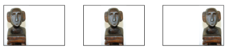
Imagine that you train a network to recognize pictures of a statue. If you trained this network on pictures where statues are near the left of the images and later try to generalize the network to pictures where statues are in the middle or to the right of an image, chances are it won’t recognize that there’s a statue there. And that’s because a vanilla neural network is not translationally invariant.
Things are different for CNNs.
Want to learn how to build modern software with LLMs using the newest tools and techniques in the field? Check out this free LLMOps course from industry expert Elvis Saravia of DAIR.AI!
Translational Invariance
What makes CNNs so powerful?
Their power lies in the ability of the network to achieve the property of translational invariance. Translational invariance is important because you’re more interested in the presence of a feature rather than where it’s located.
Once a CNN is trained to detect things in an image, changing the position of that thing in an image won’t prevent the CNN’s ability to detect it.
Anatomy of a CNN
Let’s outline the architectural anatomy of a convolutional neural network:
- Convolutional layers
- Activation layers
- Pooling layers
- Dense layers
Convolutional Layer
Instead of flattening the input at the input layer, you start by applying a filter.
Think of the filter as a “window” that you slide over small sections of an image from right to left, top to bottom, repeated over the entire image. In every one of these filters, we apply a mathematical function called a convolution. The convolution is a dot product that multiplies the different input values in that filter by some weights, adds those values up, and outputs one unique value for that window.
This process allows us to move away from individual pixels and into groups of pixels that help the network learn useful features.
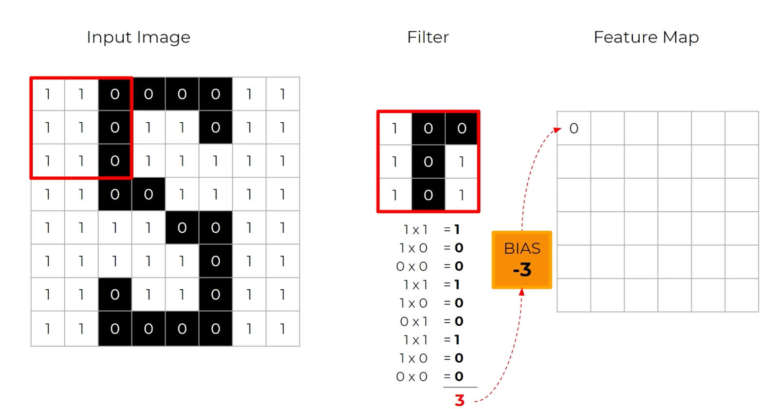
This operation is repeated for every section of the image that a filter strides over.
Because the filter is typically smaller than the whole input image, the same weights can be applied as the filter strides over the entire image. It turns out that applying the same filter to the whole image helps the network discover important features in your image. This is because each dot product gives us some notion of similarity since pixels in an image usually have stronger relationships with surrounding pixels than with pixels further away.
After repeating this process several times, you end up with a compressed version of your data called a feature map.
Activation Layer
The activation layer takes the resulting feature maps and applies a non-linear activation function — typically ReLU.
No “learning” happens in this layer, but it is still an essential component of a CNN architecture.
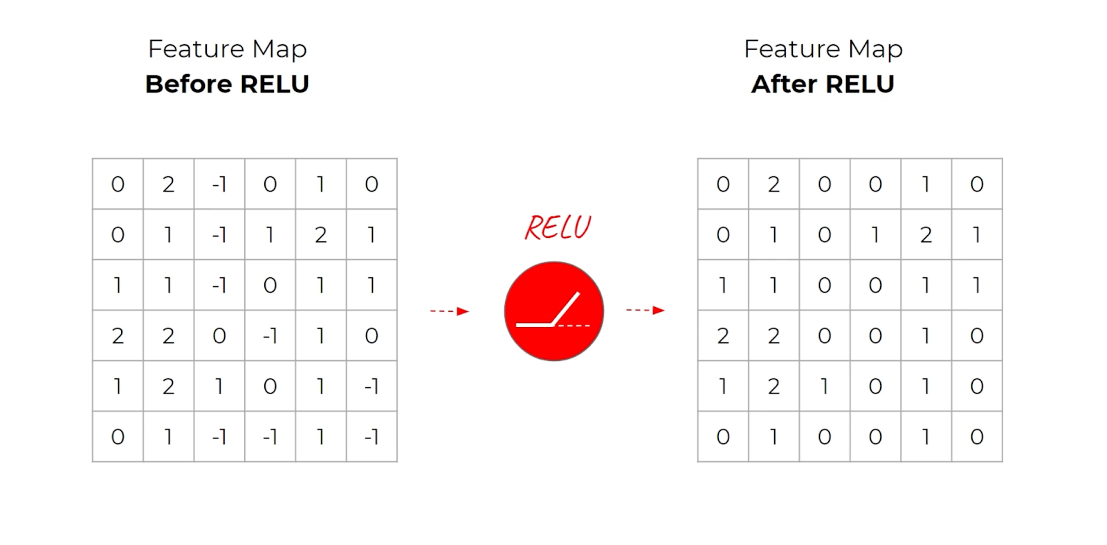
Once we have a feature map passed to an activation function, we can proceed to the pooling layer.
Pooling Layer
The pooling layer helps reduce the size of your problem space; it is essentially a dimensionality reduction.
It works by taking a grid of pixels and reducing them to a single value for future layers to receive as input. In the example below, for each 2×2 grid of pixels, the pixel with the maximum value is kept. This is called max pooling (if you wanted to you could do the average instead).

Pooling layers help control overfitting because they reduce the number of parameters and computations in the network. Since this process takes only one value of a large set of inputs and outputs, it makes it harder for the network to memorize the input. Forcing the network to learn the most important features at a more general level.
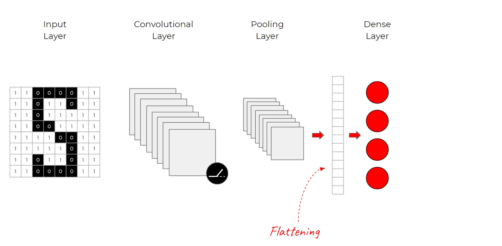
Dense Layers

By the end of this cycle of convolution, activation, and pooling layers, we flatten our output and pass it to a series of fully-connected or dense layers. The dense layers of the CNN take an input vector of the flattened pixels of the image. By this point, the image has been filtered, corrected and reduced by convolution and pooling layers.
You can then apply a SoftMax function at the output of the dense layers to provide the probability that the image belongs to a certain class.
Why Deep Networks Don’t Always Work Well
CNNs typically have several iterations of convolution and pooling layers, with some architectures stacking dozens and dozens of layers.
It turns out, though, that learning better networks is not as easy as stacking more and more layers. As you increase the depth of a network, accuracy increases to a saturation point and then begins to degrade as networks become deeper and deeper. You’re faced with issues such as vanishing and exploding gradients, degradation not caused by overfitting, and increasing training errors.
This issue is because parameters in earlier layers of the network are far away from the cost function. The cost function is the source of the gradient that is propagated back through the network. As the error is back-propagated through an increasingly deep network, a larger number of parameters contribute to the error. This causes earlier layers closer to the input to get smaller and smaller updates.
This is because of the chain rule.
The chain rule multiplies error gradients for weights in the network, and multiplying lots of values that are less than one will result in smaller and smaller values. When the gradient error comes to the first layer, its value goes to zero. The inverse problem is the exploding gradient, which happens when large error gradients accumulate during training, resulting in massive updates to model weights in the earlier layers [Source].
The net result of both of these scenarios is that early layers in the network become more challenging to train.

That is until a new convolutional neural network called Residual Networks (ResNets) emerged, which aimed to preserve the gradient.
Why We Need ResNet
Let’s imagine that we had a shallow network that was performing well.
If we were to copy those layers and their weights and stack them as new layers to make the model deeper, our intuition might suggest that the new deeper model would improve on the gains from the existing pre-trained model. If the new layers were to perform simple identity mapping — where all they were doing was reproducing the exact results of the earlier layers — then you’d expect no increase in training errors. However, that’s not the case [Source].
These deep networks struggle to learn these identity functions.
The new layers that are added either add new information or decrease error. Or, they need to add new information and increase errors. Beyond a certain point adding extra layers will contribute to an overall degradation in model performance [Source].
The Novelty of ResNet
ResNet tackles the vanishing gradient problem using skip connections.
Skip connections allow you to take the activation value from an earlier layer and pass it to a much deeper layer in a network. This allows for smoother gradient flow, ensuring important features are preserved in the training process [Source]. These skip connections are housed inside residual blocks.
Let’s explore what residual blocks are and how they work [Source]:
- Assume you have two layers of a neural network starting with some activation X.
- X is passed through a weight matrix where some linear operator — F — is applied.
- The result — which we can call X’ = F(X) — is then passed to a non-linear ReLU activation function.
- You then apply the same linear transformation — F — to X’
- Instead of applying the ReLU non-linearity directly to the result of the preceding operation — you skip it — and add X to F(X’).
- That result is now passed to a ReLU non-linearity.

These residual blocks, with their skip connections, provide two important benefits. First is avoiding the problems of vanishing or exploding gradients. The second is enabling models to learn an identity function. The modules either learn something useful and contribute to reducing the network error, or they perform identity mapping and do nothing at all [Source]. This enables information to skip the functions located within the module.
Residual networks can be considered complex ensembles of many shallower networks pooled at various depths [Source] and have allowed us to accomplish things that were not possible before.
What ResNet Allows You To Do
Skip connections allow you to propagate larger gradients to the earliest layers in your network by skipping some layers in between.
This allows those early layers to learn as fast as the final layers. Different parts of the network are trained at differing rates on various training data points based on how the error flows backward in the network [Source]. Ultimately, this allows you to train deeper networks than was previously possible without any noticeable loss in performance [Source].
This breakthrough has allowed for some amazing results in computer vision.
Where ResNet Works Best
ResNet works exceptionally well for many computer vision applications ranging from image recognition, object detection, facial recognition, image classification, semantic segmentation, and instance segmentation.
This model architecture has seen many accomplishments, including:
- First place in the ILSVRC 2015 classification competition with a top-5 error rate of 3.57%
- First place in ILSVRC and COCO 2015 competition in ImageNet Detection, ImageNet localization, COCO detection and COCO segmentation.
- Beat VGG-16 layers in Faster R-CNN with ResNet-101 with a 28% improvement
- Efficiently trained networks upwards of 100 and even 1000 layers.
ResNets have also been instrumental in transfer learning, allowing you to use the model weights from pre-trained models developed for standard computer vision benchmark datasets.
Common ResNet Architectures
ResNet-34
ResNet-34 was the original Residual Network introduced in a 2015 research paper.
This network inserts shortcut connections in a plain network. It had two design rules:
- Layers have the same number of filters for the same output feature map size
- The number of filters doubled if the feature map size was halved to preserve the time complexity per layer.
The result was a network consisting of 34 weighted layers.
ResNet-50
The ResNet-50 architecture is based on the ResNet-34 model with one important difference.
It used a stack of 3 layers instead of the earlier 2. The building blocks were modified to a bottleneck design because of concerns about the time it took to train the layers. Each of the 2-layer blocks in ResNet-34 was replaced with a 3-layer bottleneck block, forming the ResNet-50 architecture.
This resulted in higher accuracy than the ResNet-34 model.
ResNet-101 and ResNet-152
Using more 3-layer blocks builds larger Residual Networks like ResNet-101 or ResNet-152. And with increased network layers, the ResNet-152 has much lower complexity than other deeper models.
ResNet has shown that we can effectively architect deeper and deeper networks by creating short paths from the early to later layers. There’s no doubt that ResNet has proven powerful in a wide number of applications. However, there’s a major drawback to building deeper networks: They require time. A lot of time. It’s not uncommon of ResNets to require weeks of training.
This can be infeasible for real-world applications.
What if an architecture existed that would distill this simple pattern to provide maximum flow between layers in a network?
What if we could connect all the layers directly to each other?
Introduction to DenseNet
The Densely Connected Convolutional Neural Network (DenseNet) architecture takes skip connections to the max.
ResNet performs an element-wise addition to pass the output to the next layer or block. DenseNet connects all layers directly to each other. It does this through concatenation.
Crucially, in contrast to ResNets, we never combine features through summation before they are passed into a layer; instead, we combine features by concatenating them.
— Authors of the DenseNet paper
With concatenation, each layer receives collective knowledge from the preceding layers.

Each layer receives feature maps from the preceding layers and passes its feature map to deeper layers. The output layer now has information from every layer, returning to the first layer. This ensures a direct route for the information back through the network.
As a result, we end up with a more compact model because of this feature reuse.

The concept of dense connections has been portrayed in dense blocks. A dense block comprises n dense layers. These dense layers are connected using a dense circuitry such that each dense layer receives feature maps from all preceding layers and passes it’s feature maps to all subsequent layers. The dimensions of the features (width, height) stay the same in a dense block.
[Source]
DenseNet Benefits
Because of these dense connections, the model requires fewer layers, as there is no need to learn redundant feature maps, allowing the collective knowledge (features learned collectively by the network) to be reused.
- Alleviates vanishing gradient problem
- Stronger feature propagation
- Feature reuse
- Reduced parameter count
Fewer and narrower layers mean the model has fewer parameters to learn, making them easier to train.
Advantages and Disadvantages of These Differences
DenseNet architecture, while demonstrating several significant advantages, is typically more suited to smaller or moderately-sized networks rather than very deep networks. This is primarily due to its intensive memory usage stemming from the dense connections. However, for certain applications, the benefits of DenseNet can be substantial.
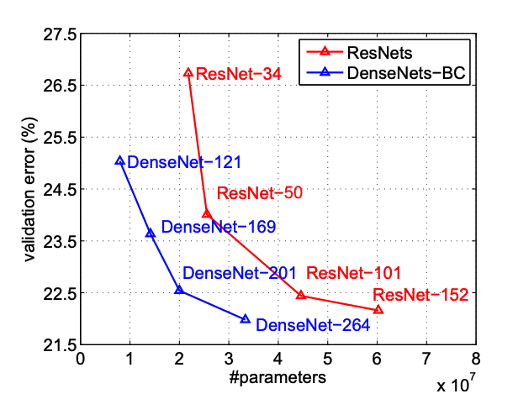
The first major advantage of DenseNet is its performance on benchmark datasets like ImageNet. The architecture has outperformed other competing architectures in terms of accuracy and efficiency. This testament to its robustness and capability in handling complex image recognition tasks.
Secondly, DenseNet’s improved parameter efficiency is a key factor in its ease of training. Unlike other architectures that might require many parameters to achieve high accuracy, DenseNet achieves this with a comparatively lower parameter count. This efficiency stems from its ability to reuse features across the network, reducing the need for learning redundant feature maps. This makes the network more compact and simplifies the training process, as there are fewer parameters to adjust during the learning phase.
Another aspect where DenseNet shines is in its resilience to the vanishing gradient problem, thanks to its dense connections. Each layer receives gradients directly from the loss function and subsequent layers, making it easier to train deeper versions of these networks compared to traditional architectures.
Despite these advantages, DenseNet also has its drawbacks. One of the main challenges is computational and memory efficiency. Due to the dense connections and concatenations of feature maps from all preceding layers, DenseNets can become quite memory intensive, especially as the network depth increases. This can make them less feasible for deployment on devices with limited resources or for applications requiring real-time processing.
Additionally, while DenseNets have fewer parameters, they can still be susceptible to overfitting, especially when trained on smaller datasets. It’s important to implement appropriate regularization techniques, such as dropout or data augmentation, to mitigate this risk.
DenseNet vs ResNet
When comparing DenseNet with ResNet, several key differences stand out:
- Skip Connections: ResNet uses skip connections to implement identity mappings, allowing gradients to flow through the network without attenuation. DenseNet, on the other hand, uses dense connections, concatenating feature maps from all preceding layers.
- Memory Usage: DenseNets generally require more memory than ResNets due to the concatenation of feature maps from all layers. This can be a limiting factor in certain applications.
- Parameter Efficiency: DenseNet is often more parameter-efficient than ResNet. It reuses features throughout the network, reducing the need to learn redundant feature maps.
- Training Dynamics: DenseNets might have a smoother training process due to the continuous feature propagation throughout the network. However, this can also lead to increased training time and computational costs.
- Performance: Both architectures have shown exceptional performance in various tasks. ResNet is often preferred for very deep networks due to its simplicity and lower computational requirements. DenseNet shines in scenarios where feature reuse is critical and can afford the additional computational cost.
Advantages and Disadvantages of These Differences
The main advantage of DenseNet’s architecture is its efficiency in reusing features and reduced parameter count. This can lead to more compact models that are powerful yet simpler to train. However, the downside is the increased computational and memory requirement, which might not be suitable for all applications, especially those with resource constraints.
ResNet’s main advantage lies in its ability to facilitate the training of very deep networks through skip connections, which mitigate the vanishing gradient problem. Its architecture is more straightforward and often more computationally efficient than DenseNet. However, it might not be as efficient in feature reuse, potentially requiring more parameters to achieve similar performance.
Conclusion
In summary, both ResNet and DenseNet offer unique advantages and have their specific use cases in deep learning. The choice between the two depends on the specific requirements of the task at hand, including computational resources, network depth, and the need for parameter efficiency. Understanding these architectures and their differences is crucial for any deep learning practitioner looking to leverage the latest advancements in CNNs for their applications.
Related Articles

